London R5R Model and Large Datasets

The workshop files also includes an R5 model of London. This is a much larger model and is more computationally intensive to use than the Montreal model, so you might need to use a desktop machine to get the most out of this.

The workshop files include the following June 2023 GTFS data, converted using the UK2GTFS tool-

London.zip – All the tube, bus, overground and tram services.
NationalRail.zip – heavy rail services from main line stations such as King’s Cross and London Bridge. Note that most of South London is covered by National Rail services as there are few tube lines here.
SouthEast.zip – Bus services in the South East region, covering towns such as Reading and Brighton. This file is only needed if you want a bigger regional commuting model.
EastEngland.zip – Bus services in East of England / East Anglia region, covering towns such as Southend and Norwich. This file is only needed if you want a bigger regional commuting model.

The more services are included, the more comprehensive the model is, but also the slower it will run. So if you are only interested in bus and tube services within London then any models you build should include the London GTFS data and ignore the rest. National Rail will be needed for many London studies given how important it is in South London and the wider South East region. The SouthEast and EastEngland files are probably not needed for most projects.

The workshop files include a network.dat file compiled using the London and NationalRail GTFS files, as well as the street network. This file is 1.3gb, so we can see how studying a larger network is going to be more computationally demanding.

Let’s do some basic accessibility analysis with the London model. Close the Montreal model, and restart R. Firstly we need more RAM this time, for example 10gb. This is particularly the case when building a new network, though in this instance we are using a network that has already been built-

options(java.parameters = "-Xmx12G")

Then load the libraries again-

library(r5r)
library(sf)
library(data.table)
library(ggplot2)

And setup the London model with the folder where you have unzipped the London files-

r5r_core <- setup_r5(data_path = "C:/Accessibility/London/")

As we have the network.dat file setup, then this should be quick.

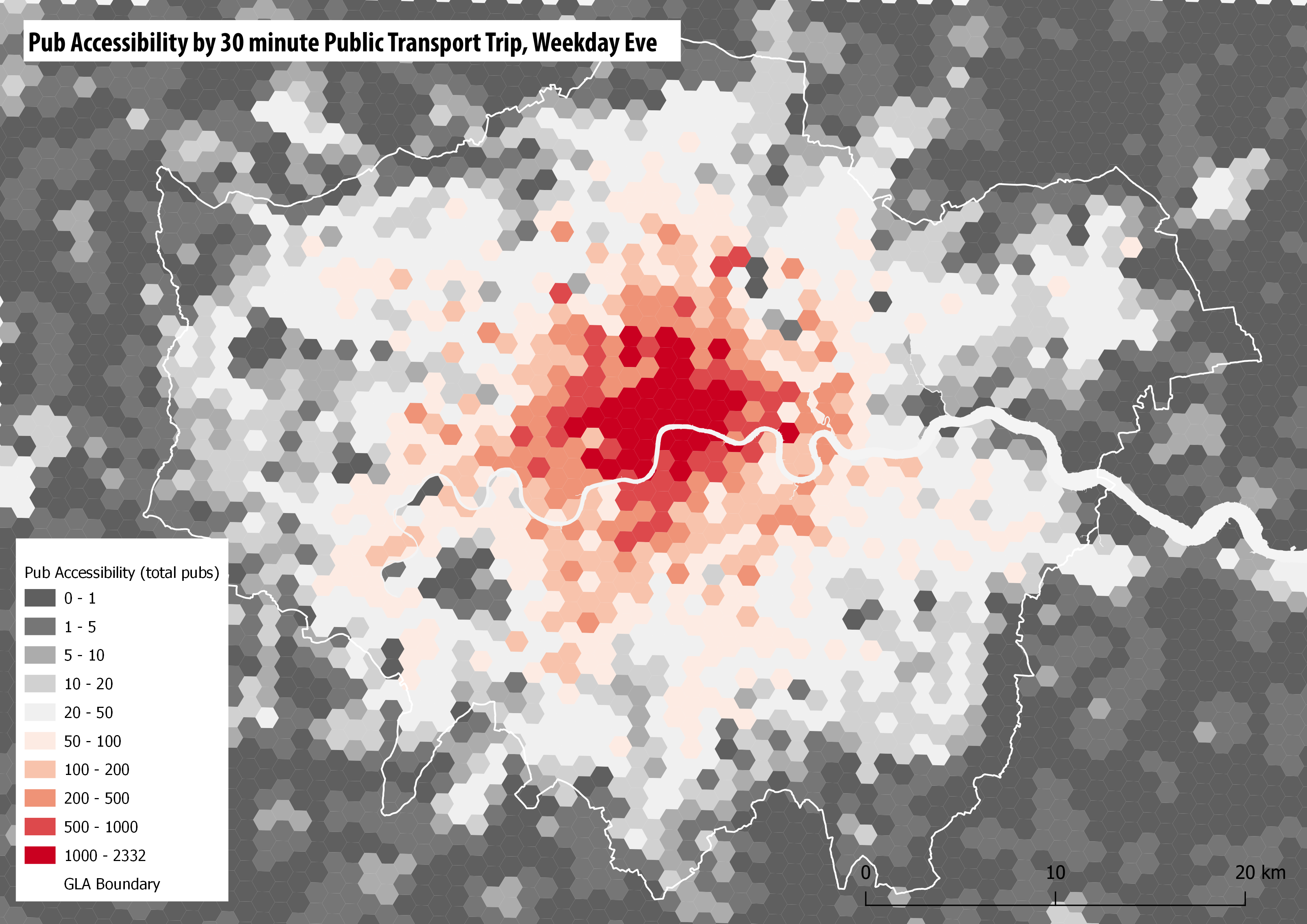
As last time, the choice of origins and destinations has a significant influence on computation time. Here we will use a 1km grid of origin points (centroids of hexagons) to retail Points of Interest destinations-

orgpoints <- fread(file.path("C:/Accessibility/London/HexGrid_1km.csv"))
destpoints <- fread(file.path("C:/Accessibility/London/LondonPubs.csv"))

And then set up the query properties as before. Note we are changing the departure date to match the time period of our GTFS files, and time to look at evening accessibility for pubs and bars-

mode <- c("WALK", "TRANSIT")
max_walk_time <- 30 # in minutes
travel_time_cutoff <- 30 # in minutes
departure_datetime <- as.POSIXct("07-06-2023 18:00:00", format = "%d-%m-%Y %H:%M:%S")
time_window <- 30 # in minutes
percentiles <- 50

Finally, we can run our accessibility query based on those settings-

access <- accessibility(r5r_core,
                        origins = orgpoints,
                        destinations = destpoints,
                        mode = mode,
                        opportunities_colnames = c("pub"),
                        decay_function = "step",
                        cutoffs = travel_time_cutoff,
                        departure_datetime = departure_datetime,
                        max_walk_time = max_walk_time,
                        time_window = time_window,
                        percentiles = percentiles,
                        progress = TRUE)

This query will take a bit longer than the Montreal model, but should be no longer than a few minutes as we used a more sparse 1km grid for the origins. If you use a denser grid of origin points then these queries can easily take hours to run. Ways to manage this include- using an intermediate grid resolution (e.g. 500m, 400m); including all your destinations in a single query (the number of destinations has much less impact on the query time); splitting up your origins into separate files, e.g. a different origin file for each London borough.

Output your results as before by exporting to a CSV file-

write.csv(access, "C:/Accessibility/London/PubsAccess30m.csv", row.names=FALSE)

Then this CSV file can be joined to the London Hex Grid file and mapped in QGIS-

We can also repeat the nearest hospital analysis with the London model. The Point of Interest data is from the Ordnance Survey POI, which enables specifying hospitals with Accident & Emergency services. You can see that Greater London has good hospital coverage-

Building a Regional Model of the South East
We can also try to build a larger commuting model of the South East, including the GTFS files for the East of England and South East regions, and a larger street network. An example output of this is shown below, with travel times to King’s Cross station during the morning peak. This model produces some interesting results, but inevitably is more computationally demanding to run. The map shows the main rail services from King’s Cross and St Pancras, such as rail links going north to towns such as Luton and Stevenage, and Thameslink going south to Crawley and Brighton. You can also pick out HS1 to Dartford and Ashford in Kent.

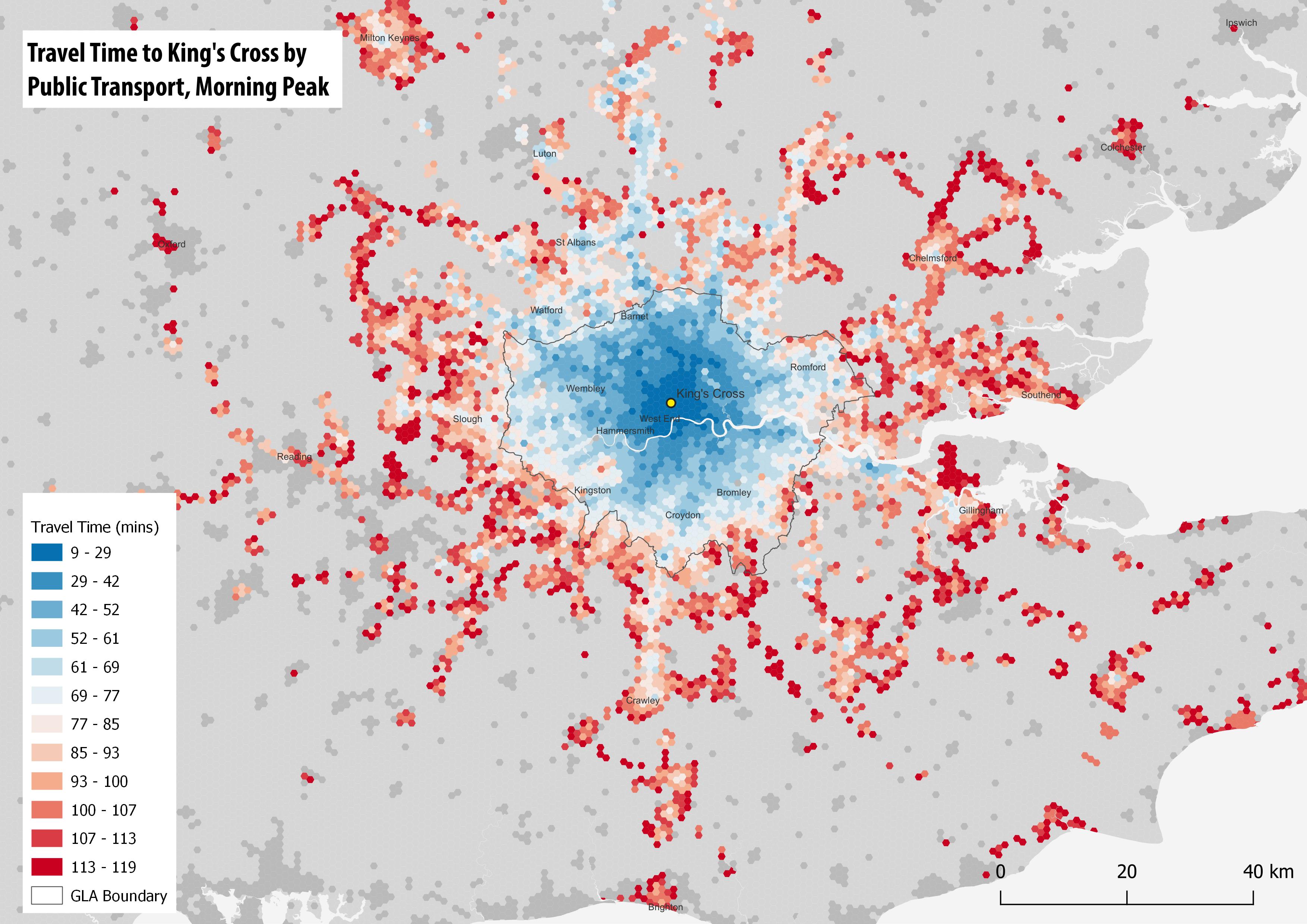
When you build a larger model, there are more likely to be some errors. So in the above map, Reading to the west looks too low density, perhaps because the train station has not linked successfully with the street network, or local bus services are not being captured. These are the kind of issues you might have to try and sort out in your model.

Workshop Pages–

Share this: