Now that we have our street network, transit schedule and point datasets ready, we can do some accessibility analysis using r5r. You should already have installed r5r-
install.packages("r5r")
And assigned some more RAM to Java, at least 2gb for this example, 5gb is ideal.
options(java.parameters = "-Xmx5G")
Next we have to load the r5r library and a few related dependencies-
library(r5r)
library(sf)
library(data.table)
library(ggplot2)
Building the Network Dataset
R5r takes the street network and GTFS datasets and processes these to create a network.dat file. This step is only required the first time we load a city model. The next time we can use the network file created the first time. So the first time the model is run it can be slow. Additionally, the first time you run r5r it will download the JAR file for R5 which will further slow down the first run (this is cached for future use).
To build the Montreal model, run the following command, using the directory of where you are storing your data files-
r5r_core <- setup_r5(data_path = "C:/Accessibility/Montreal/")
This will take a couple of minutes the first time your run this command. You should get messages stating that the JAR file has been downloaded and that the network.dat file has been created. You will also get a string of error messages related to minor issues with the street network data such as problems with turn restrictions. These generally relate to driving and are not an issue (though it is worth keeping an eye on the error messages in case there are more serious problems with the street network or GTFS data).
Accessibility Example- Access to Supermarkets
For our first example, we will count the number of supermarkets that can be reached in 30 minutes travel time by transit and walking modes in Montreal. We do this with the accessibility function in r5r. First of all we need to set up our origin and destination points, and the properties of the query.
There are a lot of different options when calculating accessibility, including the travel modes, the travel time, the origins and destinations. Additionally we have the type of accessibility we are calculating (we will do the simplest cumulative accessibility here), and the time window in r5r. Setup the following options-
mode <- c("WALK", "TRANSIT")
max_walk_time <- 30 # in minutes
travel_time_cutoff <- 30 # in minutes
departure_datetime <- as.POSIXct("12-04-2023 08:00:00", format = "%d-%m-%Y %H:%M:%S")
time_window <- 30 # in minutes
percentiles <- 50
The mode controls which modes we allow in the trip. TRANSIT includes all public transport options (TRAM, SUBWAY, RAIL, BUS, FERRY, CABLE_CAR, GONDOLA, FUNICULAR) excluding taxis. You specify these individually to see the role of public transport modes in isolation. In addition to transit modes, R5 includes WALK, BICYCLE, CAR, BICYCLE_RENT and CAR_PARK modes.
Max walk time is the maximum distance we will allow travellers to walk. The travel time cutoff is the maximum trip duration we are going to consider in the query. The cutoff can also be expressed as a list of multiple travel times (see hospital example below). Departure date needs to correspond to the GTFS files being analysed.
The R5 model handles time in a sophisticated way to address the issue that accessibility can change minute by minute depending on how your departure time aligns with the schedule of infrequent services. We specify both a departure time and a ‘time_window’ – the analysis will test multiple trip times across that time window (several for every minute), producing a distribution of travel times from which we take percentile (specified in the percentiles variable). This minimises errors from the Modifiable Temporal Unit Problem.
Then we need to set up our origin and destination points, in this case our 1km grid and our supermarket POI data-
orgpoints <- fread(file.path("C:/Accessibility/Montreal/PopGrid1km.csv"))
destpoints <- fread(file.path("C:/Accessibility/Montreal/POI.csv"))
Finally, we can run our accessibility query based on those settings-
access <- accessibility(r5r_core,
                        origins = orgpoints,
                        destinations = destpoints,
                        mode = mode,
                        opportunities_colnames = c("supermarket"),
                        decay_function = "step",
                        cutoffs = travel_time_cutoff,
                        departure_datetime = departure_datetime,
                        max_walk_time = max_walk_time,
                        time_window = time_window,
                        percentiles = percentiles,
                        progress = TRUE)
This will take a couple of minutes to run. On completion, the results are passed to the data table ‘access’. You can check the contents of the access table by running head(access). Finally export the access data as a CSV file-
write.csv(access, "C:/Accessibility/Montreal/SupermarketAccess30m.csv", row.names=FALSE)
Mapping the Supermarket Accessibility Data
The output of the accessibility query is the total number of supermarkets reachable in a 30 minutes transit and walking trip for each of our origin points. This data could be mapped directly within R using a library such as ggplot. Or alternatively it can be mapped in QGIS, as shown below. This has been achieved by joining the SupermarketAccess30m.csv file to the original point grid MontrealGrid_1km (found in the Geopackage Montreal in the workshop files). Then we classify the points. The output shows excellent accessibility in central Montreal and variable access in the suburbs depending on the geography of metro lines and bus services.

Travel Time to the Nearest Facility Query
The above query type of totalling the number of opportunities within a travel time threshold makes sense for services such as retail where choice and the number of opportunities is important. For other public services, the priority can be less about choice and more about minimising access time to the nearest facility. This is the case for hospital accessibility. In the next example we will use the same accessibility function and tweak some settings. R5R does not natively calculate access times to the nearest facility, but we can approximate this analysis by testing multiple travel times in the cutoff variable-
travel_time_cutoff <- c(10,20,30,40,50,60,70,80)
Then we can repeat our accessibility function, this time switching the opportunity column from supermarkets to hospitals-
access <- accessibility(r5r_core,
                        origins = orgpoints,
                        destinations = destpoints,
                        mode = mode,
                        opportunities_colnames = c("hospital"),
                        decay_function = "step",
                        cutoffs = travel_time_cutoff,
                        departure_datetime = departure_datetime,
                        max_walk_time = max_walk_time,
                        time_window = time_window,
                        percentiles = percentiles,
                        progress = TRUE)
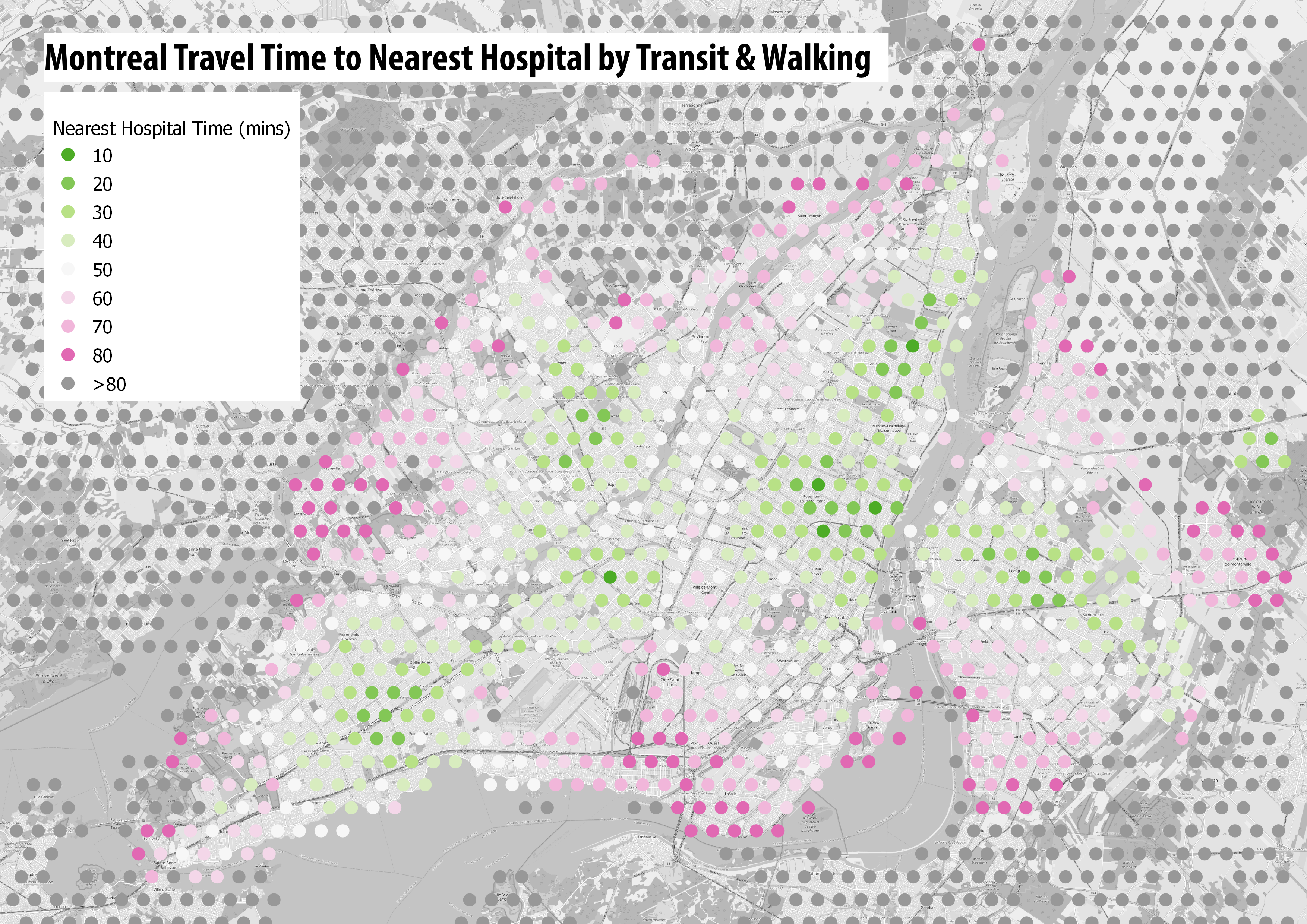
This time the output will include 1 row for each travel time included (10,20,30…). Therefore to find the minimum travel time, we need to do a group by function for all rows where hospital > 0, and find the minimum cutoff value. In the example below, the minimum cutoff query was done in QGIS using the Statistics by Categories function. The location of major hospitals in the city can be clearly seen in the map below, with some areas of poorer accessibility such a south of the city centre.
As well as mapping this data, we can also calculate some basic statistics using the population data that is linked to each origin point, such as the graph below-

Next we will explore the travel time matrix function-
Workshop Pages–
- R5R Accessibility Workshop Intro
- Getting Started & Installation
- Transit Schedule & Street Network Data
- Accessibility Example 1 – Access to Facilities: Retail & Hospitals
- Accessibility Example 2 – Travel Time Matrix and Isochrones
- UK Transit Data – TransXchange & ATOC
- London in R5 and Modelling Large Cities
- Accessibility Analysis Further Resources
