In the previous section we looked at the accessibility function, which summed an opportunity column within travel time thresholds. Next we will look at the travel_time_matrix function, which will return travel times between the origin and destination points that we specify.
We are going to test this by calculating travel times from a single origin, the Gare Centrale (Central Station) in Montreal. The travel time matrix function can be used to calculate travel times from all origins to all destinations. This will inevitably be a much more computationally intensive and slower query. The way R5 works, it is the number of origins that most influences how long the query takes. So travel times from a small number of origins to many destinations is a much faster query than many origins to few destinations. For this initial test, try the following origins and destinations-
orgpoints <- fread(file.path("C:/Accessibility/Montreal/Station.csv"))
destpoints <- fread(file.path("C:/Accessibility/Montreal/PopGrid1km.csv"))
The query settings are very similar to the access function, but this time we create a max_trip_duration variable rather than a travel_time_cutoff. We will cap the travel time matrix at 2 hours or 120 minutes.
mode <- c("WALK", "TRANSIT")
max_walk_time <- 30 # in minutes
max_trip_duration <- 120 # in minutes
departure_datetime <- as.POSIXct("12-04-2023 08:00:00", format = "%d-%m-%Y %H:%M:%S")
time_window <- 30 # in minutes
percentiles <- 50
We can now run the travel time matrix function-
ttm <- travel_time_matrix(r5r_core,
                          origins = orgpoints,
                          destinations = destpoints,
                          mode = mode,
                          departure_datetime = departure_datetime,
                          max_walk_time = max_walk_time,
                          max_trip_duration = max_trip_duration,
                          time_window = time_window,
                          percentiles = percentiles,
                          progress = TRUE)
The output is stored in the ttm data table. We can export this as a CSV file-
write.csv(ttm, "C:/Accessibility/Montreal/StationTTM.csv", row.names=FALSE)
The map below shows the output of this query in QGIS, where the travel time matrix is joined to the original points file. Note this map uses the 100m Pop Grid file rather than the 1km Pop Grid file, so the map resolution is higher and you can see more details, such as how bus services run along main streets linking to the metro lines-
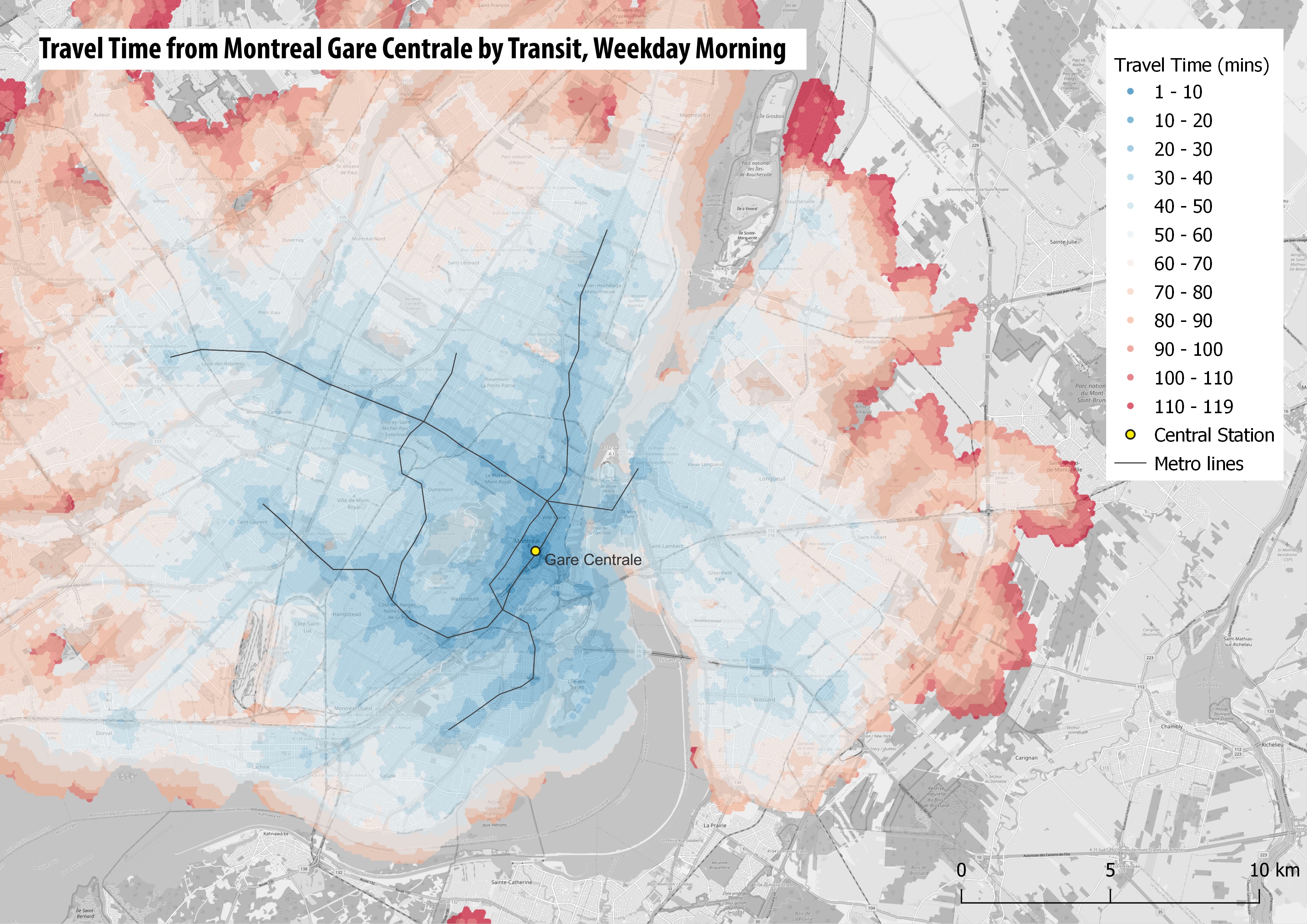
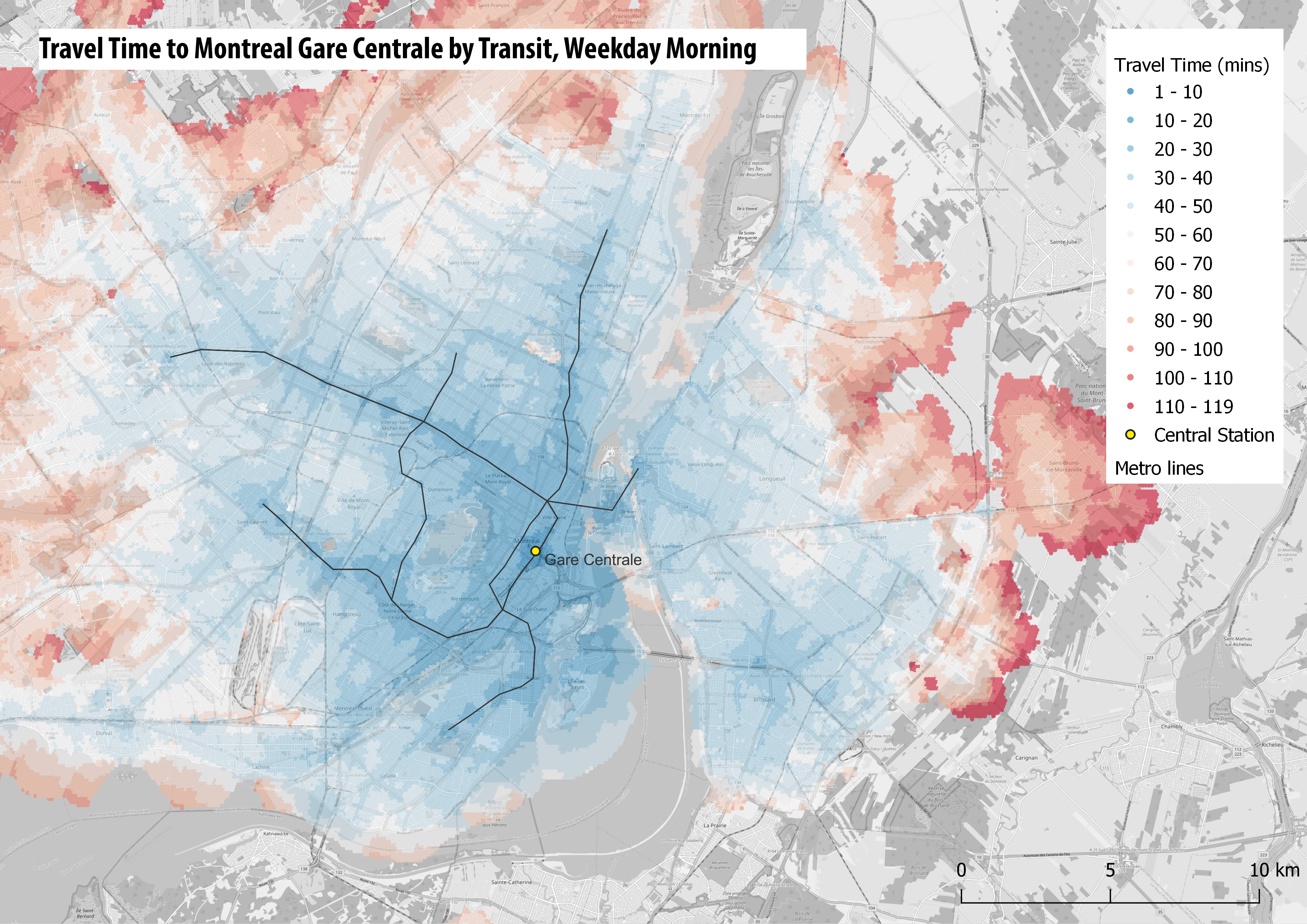
If you remember at the start we specified Montreal Central Station as the origin, and the population points as the destinations. We can swap these over to get a more realistic query for commuting into the city centre during the morning peak. Due to the way R5 works this is a slower query (around 30 minutes calculation time), and you can use the results file provided in the workshop files, StationTTM.csv. The results are show below. While the to and from maps are largely similar, you can if you look closely see that the accessibility to Gare Centrale is better than accessibility from Gare Centrale. Like most cities, commuter services are prioritised inbound during the morning peak-
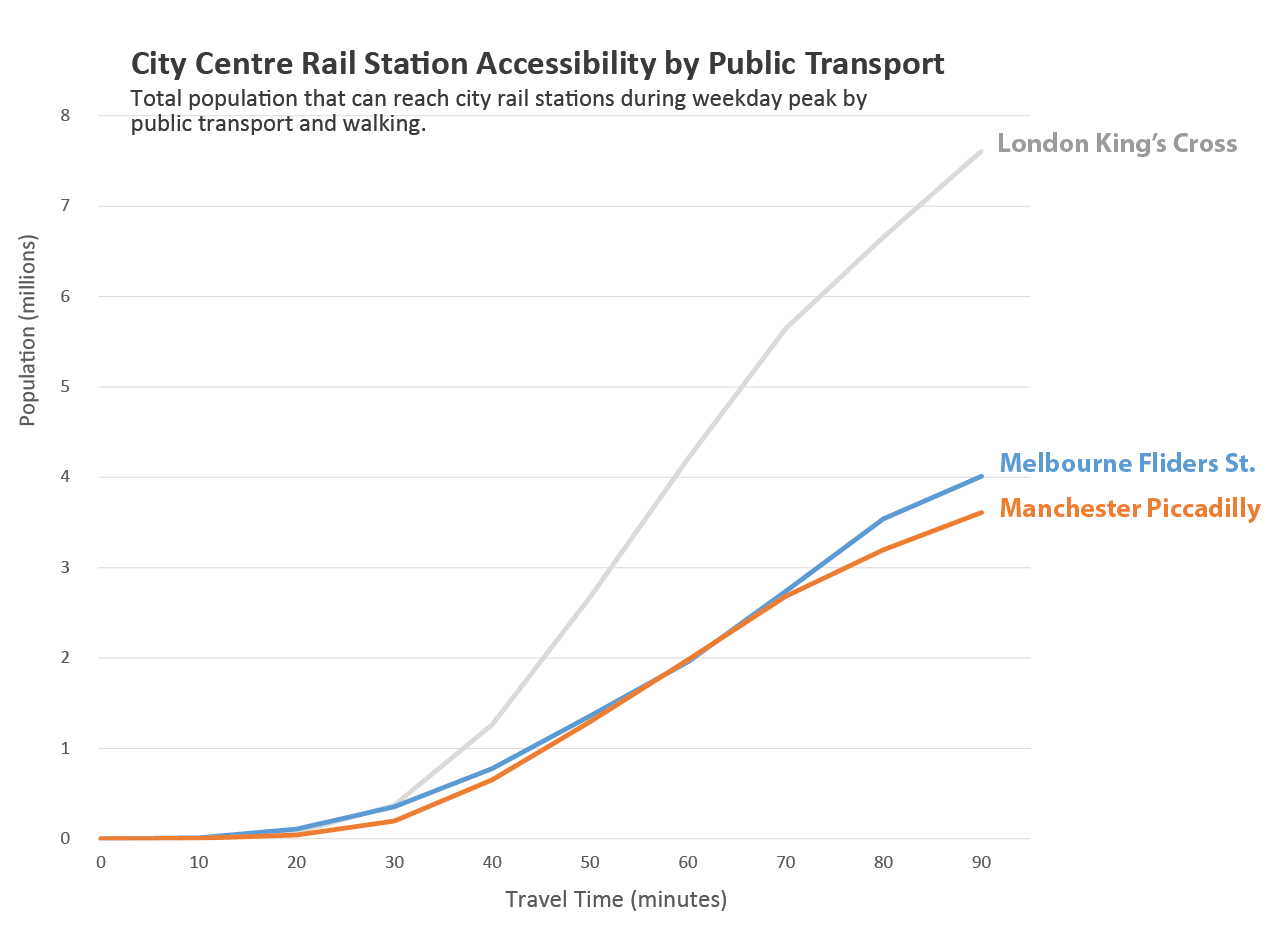
The travel time matrix can be analysed statistically as well, for example comparing population accessibility by public transport to city centres in different cities-
Next we are going to discuss using UK public transport data in R5.
Workshop Pages–
- R5R Accessibility Workshop Intro
- Getting Started & Installation
- Transit Schedule & Street Network Data
- Accessibility Example 1 – Access to Facilities: Retail & Hospitals
- Accessibility Example 2 – Travel Time Matrix and Isochrones
- UK Transit Data – TransXchange & ATOC
- London in R5 and Modelling Large Cities
- Accessibility Analysis Further Resources
